K-means and KD-trees resources
- Read the K-means paper (PS),
or K-means paper (PDF) .
- Note:
recently a similar, though independent, result, was brought to our
attention. It predates our work. For completeness, you can read that
too.
- Read the X-means paper (PS)
or X-means paper (PDF).
- The X-means and K-means implementation in binary form
is now available for download! Currently, there are versions for
linux, OS X, and MS-Windows. They are distributed under the following
terms:
- The software may be used experimental and research purposes
only.
- The software may not be distributed to anyone else, and may not
be sold in whole or within part of a larger software product, whether in
source or binary forms.
To download it, simply get the file appropriate for you at the
kmeans download section.
- X-means is available to researchers in source form. The code is
in standard C, and can be run standalone or via a MATLAB wrapper. It
is known to compile under GCC (on Linux, Cygwin, OS X, Solaris, and FreeBSD)
and MSVC++.
- In addition to X-means, this code also includes fast K-means support.
It will accelerate your K-means application, provided that:
- Your data has no more than 15 dimensions. You can still get and use the
code if this doesn't hold, but don't expect it to be particularly fast. The
code includes a straightforward implementation of K-means that doesn't use
KD-trees.
- You can compute Euclidean distances between any two of
your data points, and this distance is meaningful in some way to you. This
is actually a prerequisite of any K-means algorithm.
- To obtain access, fill the blanks in this License
Agreement, and mail it back to Dan Pelleg (yes, there's a plus
sign in there; just leave it and the words before and after it like they
are - it works). Basically, all it says is that you can't use this program
commercially. You're welcome to request it - I granted around 800 licenses
already to people in as many institutions and am always glad to have more
users. I will not sell, rent, give away or otherwise use your email address
for any purpose other than to give you the download instructions.
- There is also a
K-means and
X-means mailing-list.
- Below, I prepared a "cartoon guide" to K-means:
Introduction to K-means
Here is a dataset in 2 dimensions with 8000 points in it. We will run
5-means on it (K-means with K=5). In addition to the points we see
K-means has selected 5 random points for class centers. This are the fat
blue, green, red, black, and purple points. Notice that, as chance has it,
they do not correspond to the underlying Gaussians (as a matter of fact I
had to coerce the program to produce those "bad" initial points - it is
fairly good at getting the initial points "right").
Now, the program goes over datapoints, associating each one with the class
center closest to it. The points you see are colored according to the center
they're associated with. Notice the blue-green boundary at the top
right-hand corner. This (theoretical) line of points which are equidistant
from the green and blue centers determines which point belongs where.
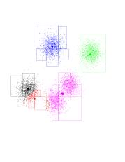
The next step of the algorithm is to re-position the class centers. The
green center will be placed at the center of mass of all green points, and
so on. As it turns out, the green center will shift to the right and
upwards. The black line going out from the green center shows this. Notice
the black and red centers each share about half of the Gaussian on the left
(and about a half of the Gaussian they're in), so they both "race" to the
left. The purple center's movement is very small.
Click on the image to see a larger version. You can open it in a new
browser window, so you can still read the text.

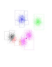
The program moved the centers, and re-colored all points according to which
center is closest to each. Since the green center has moved, the blue-green
boundary passes "outside" of the Gaussian on the top-right-hand corner. And
is probably somewhere in the unpopulated area between blue and green. We
want this kind of thing to happen.
By looking at the movement vectors, you can see the black and red will
continue racing to the left, and the purple now dominates a good part of its
surroundings. Notice the "orphan" Gaussian between purple and green. This
happened because black and red reside in the same Gaussian, so we're "short"
one centroid.

The green-purple boundary shifts upward and to the right; looks like green
is going to own just "its" points and purple will own two Gaussians. On the
bottom left-hand corner, it looks like red had lost the race to black
(black is more to the left).

Another iteration...

Now the blue-green and green-purple boundaries are pretty much set (to what
they should be). Notice that red will shift, ever so slightly, to the right.
Red has gone to the right. So it gained more purple points. Since all of
the purple points are to its right, this effect intensifies. Consequently,
purple is losing points to the red, and moves right (and up) as well.
Another iteration...

And another one...

And another one...

The red has completed its journey, gaining control over a Gaussian
previously owned by purple. Black gets to own the entire Gaussian on the
left. K-means has found the "correct" partition. Since this is a stable
configuration, the next iterations will not move the centers too much.

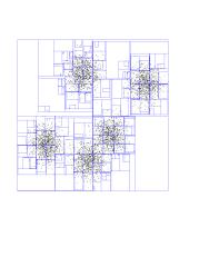
Introduction to KD-trees
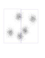
Again, our dataset of 8000 randomly-generated points, from a
5-Gaussian distribution. You should see the underlying Gaussians. The blue
boundary denotes the "root" kd-node. It encompasses all of the points.

Now see the children of the root node. Each is a rectangle, with the
splitting line parallel to the Y axis about half-way through.
Now you see the grand-children of the root. Each one is a split of its
parent, along the X-axis this time.

And so on, splitting on alternating dimensions...


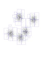


Here are the first seven layers of KD-tree, all in one picture.
Doing fast K-means with KD-trees
All the explanations in the K-means demo above were true for traditional
K-means. "Traditional" means that when you go out and decide which center
is closest to each point (ie, determine colors), you do it the naive way:
for each point, compute distances to all the centers and find the
minimum. Our program is much smarter then that. It first builds a kd-tree
for the points (the one you saw earlier). Now assume that some kd-node is
entirely owned by some center. This means that the next center
movement will be affected by the center of mass of the points in that
kd-node (and their number). So, by pre-computing the center of mass of each
kd-node, and storing it in the node, we can save a lot of work. [showing
that some node is entirely owned by a center can also be done efficiently
-- see the fast K-means paper].
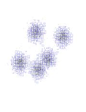
This kind of fast computation has been going on behind the scenes
throughout the demo. Whenever a node was proven to be fully owned by a
center, the program drew that node's rectangle. For visualization purposes
it also drew the points inside it, but a "real" program doesn't need to do
that. It just uses a very small constant number of arithmetic operations to
compute the effect a certain kd-node will have. This is opposed to summing
the coordinates of each and every point inside that rectangle, that is, a
cost which is linear in the number of points in the rectangle.
Notice how easy it was to compute the black and blue centers-of-mass. The
black took just two nodes, and about 50 additional individual points. The
blue took 5 nodes, plus about 10 points. Compare this with the roughly
8000/5 = 1600 points each one has (and doing 5 distances for each!).
Another interesting thing to notice is how these rectangles get smaller as
we approach the theoretical boundary line we talked about before. Watch the
red-purple boundary. As we get closer to it, it's harder and harder for
big, fat nodes to be owned entirely by either red or purple. If you think
about it, they can't be owned entirely by either center if this boundary
intersects them. So, the closer we get to the boundary, the smaller the
rectangles. And it's pretty much individual points very close to the
boundary.
Maintained by Dan Pelleg.
This material is based upon work supported by the National Science Foundation under Grant No. 0121671.
View this page in Romanian courtesy of azoft.
![[Back arrow]](images/back.gif) Back to my home page
Back to my home page
Last updated: 2012/08/01 18:23:56