Proceedings of the IEEE Symposium on Information Visualization (InfoVis '99), San Francisco, CA, October, 1999, pp. 84-91.

Efficient Multi-Object Dynamic Query Histograms

Mark Derthick, James Harrison, Andrew Moore, Steven F. Roth

Carnegie Mellon University Robotics Institute

{mad+, jaharris+, awm+, roth+}@cs.cmu.edu

Abstract

Dynamic Queries offer continuous feedback during range queries, and have been shown to be effective and satisfying. Recent work has extended them to datasets of 100,000 objects and, separately, to queries involving relations among multiple objects. The latter work enables filtering houses by properties of their owners, for instance. Our primary concern is providing feedback from histograms during Dynamic Query. The height of each histogram bar shows the count of selected objects whose attribute value falls into a given range. Unfortunately, previous efficient algorithms for single object queries overcount in the case of multiple objects if, for instance, a house has multiple owners. This paper presents an efficient algorithm that with high probability closely approximates the true counts.

1. Previous Dynamic Query work

1.1. Single Object Interface

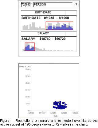
Figure 1 shows a Dynamic Query (DQ) interface as implemented in VQE, a Visual Query Environment for exploring data from a database [1]. VQE is built on top of Visage [2], an interactive data visualization system developed by Carnegie Mellon and Maya Design Group.

The subset of the database being explored at any given time by a VQE query is called the active subset. The top row in the upper box of Figure 1 indicates that the query is being applied to an active subset of 195 people, and that 72 of these people satisfy the constraints imposed by the sliders on the remaining two rows. Namely, they have a birthdate between 8/1935 and 8/1968 and a salary between $15,760 and $66,729. The rectangular sliders are superimposed on histograms where the dark bars show the distribution of the attribute values for the 72 selected people. The dark bars partially cover the light bars, which show the distribution for all 195 people. When the user drags either end of the sliders to change a query’s selection range, the counts, histograms, and visibility of the points in the chart are updated in real time. In Figure 1, the attributes shown on the axes in the chart are the same ones being filtered, so data only appears in a small rectangular area.

1.2. Efficient Algorithms

We will only describe algorithms for updating the histograms. The counts in the top row of the upper box in Figure 1 can be implemented as a zero dimensional histogram. The chart can be implemented as a 2D histogram where the pixel at xy is turned on if the count for that histogram bucket is greater than zero. For the following algorithms let

a number of sliders

p slider width in pixels

r number of objects in active subset

The sliders' edges can be positioned at any of the p pixel positions. Even though the histogram bars as displayed are several pixels wide, the histograms are computed with p buckets internally. Several of these buckets are then added when computing the bar heights for display.

After every mouse move drags a slider edge, the screen should update within 0.1s in order to feel like continuous feedback [3]. Several schemes have been presented to avoid scanning the entire active subset in raw form after each mouse move, by preprocessing to create index data structures. Preprocessing can occur after any of four event types. The higher level the event, the more time is available without annoying the user. The first two numbers come from formal experiments [3], the third from informal observation [4], and the last from the observation that data warehouses are typically updated daily and that it would be reasonable to run an indexing program overnight.

mouse move	0.1s
mouse down	1 s
active subset selection	10 s
data warehouse update	10,000 s

Previous Dynamic Query indexing algorithms have been restricted to records from a single relational database table, which we call `single object queries.’ In order to explain the reasons for our design decisions and where previous algorithms break down, we first describe in detail a previous mouse-down indexing algorithm and kd-tree based active subset selection algorithms. While necessary for an understanding of the tradeoffs among these indexing schemes, the reader can skip to section 1.3 without major loss of continuity.

TBS Algorithm

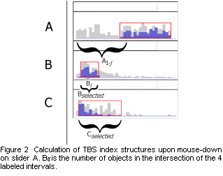
Tanin, Beigel, and Shneiderman [4] present a mouse-down indexing algorithm that we will call TBS. As soon as the user depresses the mouse button to begin dragging slider A, the active subset can be filtered to remove objects based on sliders B, C, etc. Further there are only a limited number of possible updates to allow for, since the mouse can only move to the few hundred pixels of slider A. For every bucket of slider A, B, C, etc an index structure is created for quickly calculating the number of selected objects in the bucket. The index structure for bucket B_i is an array of length p, where B_ij is the number of objects whose B attribute falls into bucket i, whose A attribute falls into one of buckets 1-j, and whose B, C, etc attribute falls into the selected range for that attribute (see Figure 2). Then when the mouse moves, the count is updated to B_i = B_{i right} - B_{i left} , where right (left) is the pixel index of the right (left) edge of slider A. This gives the number of objects whose A attribute is greater than the left cutoff but less than the right cutoff. This subtraction must be done for each bucket of each slider, so the complexity of updating the histograms is just O(ap). Since this is independent of r, moving the mouse is very fast. The bottleneck is creating the index structures.

Computing the index structures requires looking at each attribute of each object, which takes O(ar) time. If its B, C, etc attributes fall within the selected ranges, then the appropriate B_ij is incremented. This produces non-cumulative B_ij. The final, cumulative, B_ij are computed by looping through each i and j for each slider B, C, etc, taking O(ap²). The total time for computing index structures is therefore O(ar+ap²).

TBS with kd-trees

As future work, Tanin, Beigel, and Shneiderman [4] suggest that a kd-tree can be built at active subset selection time so that sequential scan is not necessary in order to build the structures above. A kd-tree is a binary tree whose root represents all r objects. Each node of the tree divides its set of objects approximately in half by thresholding on some attribute. It always chooses the attribute with the maximum range of values over the node’s objects, relative to its range for the entire active subset. If the range falls within a single histogram bucket on all attributes, it is a leaf node. Each node maintains a count of the number of data objects it owns, and the max and min value of each attribute over these objects. The number of leaf nodes is limited both by the number of objects and the cross product of all the histogram buckets, so the space complexity is O(a min(r, p^a)). The time to build the tree is O(ar log r) [5].

When building the index structures on mouse-down, the tree is traversed top-down. Nodes whose attribute ranges are disjoint from the ranges of one of the sliders B, C, etc can be pruned without looking at their children. The counts of nodes whose ranges fall within a single A bucket and a single B bucket are added to the (not yet cumulative) B_ij without looking at their children.

For portions of the tree in the selected set, every leaf node must be visited for exactly one of the histograms – the one for the attribute its parent thresholds on. At each node, the range of each attribute must be compared with the slider ranges. So the worst-case performance is O(ar), the same as for sequential scanning. But if some of the sliders B, C, etc are restricting the selected set, the time will be reduced proportionally. It will also be reduced if multiple objects fall into the same leaf node due to small p^a or skewed data.

kd-trees without TBS

For reasons explained in Section 2.2, the TBS algorithm is not practical for multi-object queries. However, kd-trees can still be used to compute histograms directly. In this case, nothing is done at mouse-down time. At mouse-move time, the tree is traversed top-down as before. The bucket count for B_i is the count in the intersection of B_i with A_selected, B_selected, and C_selected (see Figure 2). This still takes time O(ar).

For an additional factor of a in space and build time, every histogram bucket can store its own kd-tree. Then its bucket count is found with an independent range counting-query on an a-1 dimensional kd-tree. A range counting-query on an a dimensional kd-tree takes O(r^1-1/a) [6]. Each tree will have, on average, r/p objects. Performing range counting-queries for every bucket therefore takes O(ap(r/p)^1-1/(a-1)) = O(ap^1/(a-1)r^1-1/(a-1)). Subjectively there seems no reason to provide histograms wider than a few hundred pixels, whereas it is desirable to increase r indefinitely. Thus this is a theoretical improvement. In practice it produced a significant speed up, which increased with the number of sliders and the number of objects. For 3 sliders and 1,000,000 objects the difference was a factor of 10.

It probably is not practical to use this trick with TBS, because its index structures are two dimensional compared with the histograms’ single dimension. Therefore it requires an additional a² factor in space and time to construct B_ij-specific kd-trees rather than just an additional factor of a.

Detailed studies of kd-trees for Dynamic Query found them of little help except for skewed data distributions [7]. They did not consider histogram-specific kd-trees, however. Further, real data often is skewed.

1.3. Multiple Object Interface

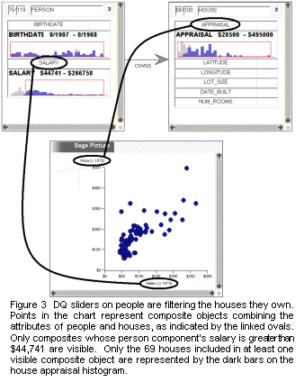
Figure 3 shows an active subset that involves the relationship between two types of objects: people and the houses they own. This sort of query is accomplished with joins in database systems. The two boxes containing counts and histograms are called nodes of the query. In general, queries can involve any number of nodes. The chart showing salary of the owner vs appraised value of the house shows composite objects that have attributes of both houses and people. By restricting the slider on the owner's salary, all composite objects containing owners outside the selected range are turned off. Thus the chart is empty to the left of $44,741. If all the composite objects containing a given house are turned off, the house is no longer counted among the selected set of houses or included in the dark bars. As can be seen in the upper right box, 69 of the 100 houses have some owner who earns more than $44,741 and remain selected. It is possible that some of the 69 selected houses also have an owner who earns less than $44,731. From the light gray bars in the Appraisal histogram it can be seen that the deselected 31 houses had appraisals near the low end of the range. By sweeping the owner salary slider to the right, the user would see that the remaining selected houses' appraisals would lie increasingly at the high end of the range. In this way DQ histograms can show correlations among multiple attributes through interaction, complementing that way the chart shows the correlation between two attributes statically.

The fact that the boxes count base level objects like people and houses grounds the displayed information in the terms the user is familiar with. The composite objects shown in the chart allow additional expressiveness by combining properties of multiple base level objects. They also allow coordination across multiple visualizations that involve different combinations of base level types. For instance if Figure 3 also contained a map showing people and their work locations, brushing a person/house plot point in the chart would also highlight the same person's work location on the map. This behavior is built into the Visage architecture. Applications built on top of Visage use a shared database and construct composite objects as needed. Cross-application brushing and drag-and-drop is falls out automatically any time their composite objects share base level components.

2. Multiple Object Counting Problem

2.1. Overview

Internally DQ must use the composite objects to build its index structures in order to constrain histograms based on sliders from multiple query nodes. Then the counts must be translated back to the base types on a node-by-node basis by removing duplicates. For instance if a house is owned by two people with salaries of $10,000 and $20,000, it must contribute a count of 1 to house histograms if the person-salary slider range includes either (or both) of these quantities. If histogram B displays an attribute of houses, such as appraisal, and if the person-salary slider A is at full width, the TBS subtraction algorithm will incorrectly compute B_ip - B_i1 = 2. Each index structure count is supposed to measure the cardinality of the set of houses that fall into a range of appraisal and person-salary. In the single object case, every object falls into exactly one B_ij so the sets are disjoint, and cardinalities of subsets can be added or subtracted. In the multiple object case, the subsets must be combined using set-union before the cardinality of the result set is computed.

Although we described the problem as it occurs in the TBS index structures, it applies equally at all the other times. Even at mouse-move time each composite object must be added to the appropriate histogram bucket, but simply incrementing a counter fails because the base object may have already been encountered in a previous composite object.

First we describe how to avoid the overcounting problem by using a bit vector representation of the sets rather than counts of their cardinalities. This approach is infeasible because it requires O(r) storage at each B_ij rather than the O(log r) required for simple counts. We then show how to use a randomized set cardinality representation that uses only O(log r) storage and with high probability gives an accurate estimate.

As an aside, Query Previews encountered a similar overcounting problem due to overlapping attribute values in their geographical domain [8]. For instance data from “North Africa” and “Libya” overlaps at every grid point in Libya. They describe a deterministic solution that relies on the fact that the areas of overlap are contiguous, so it does not apply here.

Ioannidis [9] suggests an approach that gives exact counts in the case of multi-object queries, but it requires traversing pointers among the related objects at mouse-move time, and takes O(ar) time. Our first implementation was along these lines, and was much slower than using kd-trees.

2.2. Bit Vector Set Representation

In a bit vector representation of a set, each possible element is assigned a bit position. The bit is set if and only if the set contains the element. Set union can be accomplished by bitwise OR of the bit vector representations. The cardinality is found by counting the number of bits set, which is called the weight of the bit vector. In the TBS index structure, each B_ij becomes a bit vector with bits set for all objects whose B attribute falls into bucket i, whose A attribute falls into one of buckets 1-j, and whose B, C, etc attributes fall into the selected ranges. When the mouse moves, the count is updated to B_i = weight(BITOR_{j = left to right} B_ij ). Notice that the complexity is now O(ap²), due to the cumulative BITOR over the index structure instead of a subtraction. The bitwise difference between B_{i right} and B_{i left} may undercount because a base object might show up to the left of the slider and within the slider range. Bitwise difference would remove it due to the first occurrence, even though it should be counted due to the second.

In the kd-tree for attribute B, each node maintains a bit vector with bits set for the B component of all composite objects that it owns. At mouse-move time B_i is computed by accumulating the bitwise OR of the bit vectors as the tree is traversed in the same manner as for the single object case. Since the complexity of traversing the kd-tree remains the same in the multiple object case, while the TBS algorithm slows down by a factor of p, it may no longer be a win even though it takes advantage of the factor of 10 increase in time available at mouse-down for scanning the active subset. For this reason we compute the histograms from the kd-tree directly.

Frequently the relationship between query nodes will be functional. For instance in a query about people and their state of residence, every person will have a unique state. Thus there will be a 1 to 1 relationship between people and the composite objects. In cases like these we can save a constant factor of space and time by using the numerical cardinalities in computing histograms for the people query node. Bit vectors must still be used to compute histograms for the states.

2.3. Randomized Bit Vector Representation

The bit vector representation described above is information preserving — it can be translated back to an explicit list of set elements because each potential element is assigned a unique bit position. The size of the bit vectors can be reduced by mapping multiple potential elements onto the same bit position. Information is lost, but if all we care about is cardinality, we can still estimate how many elements contributed to a given bit vector. The more bits that are set, the more elements there probably were. Using only O(log r) bits in the bit vectors, there will clearly be many collisions. If the assignment of elements to bits is equi-probable, the bit vector will quickly saturate and estimates for large cardinalities will be terrible. Flajolet and Martin [10] show that by assigning elements to bits with exponentially decreasing probability, the bit vector avoids saturation. Estimates with errors that are within a given percentage of the actual are possible. By averaging the estimates from multiple random bit vector assignments, this percentage error can be brought arbitrarily low. With V = 64 bit vectors, the error is less than 5% with high probability, independent of r [10].

Each bit vector should be of length l = ceiling(log r). To assign each object a bit, first choose a uniformly distributed random number, x, between 0 and 2^l - 1. Then compute the bit position of the first 1 in the binary representation of x. This gives a random number exponentially distributed from 1 to l, and is the bit position assigned to the object. Then randomly choose one of the V bit vectors in which to set the bit [10]. The array of V bit vectors for a kd-tree node or a TBS B_ij is accumulated by setting the bits for all the objects that belong to it in each component bit vector.

After each mouse move, when the bitwise ORed bit vector is accumulated for each histogram bucket, estimate the cardinality as follows: for each of the V bit vectors, find the bit position of the first 0 bit. Let R be the average of these bit positions over the V bit vectors. Then the estimate is 1.54703 ∙ V ∙ 2^R . The constant corrects for the bias toward undercounting inherent in the algorithm [10].

We can reduce the space further by windowing [10]. The low-order bits of the bit vectors only contribute small amounts to the estimates, and can be dispensed with. Errors that contribute less than a pixel to the height of the bars are not even detectable. If the histogram height is h pixels, we can get away with storing O(log h) bits per vector rather than O(log r).

3. Experimental Evaluation

3.1. Estimation Accuracy

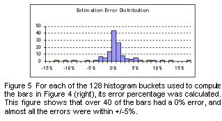
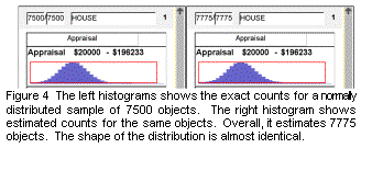
Figure 4 shows the visual impact of the estimation algorithm compared with the exact counts. There is no noticeable difference. Figure 5 shows the distribution of errors. Most bars heights are within 5% of the correct value, which corresponds to about 1.5 pixels. We subjectively conclude that 64 bit vectors offers a good compromise between efficiency and accuracy.

3.2. kd-tree Speed

We used the VQE interface to display a varying number of attributes, histogram widths, and composite objects. We used synthetic data in which each attribute is independent and uniformly distributed, which gives the worst case performance for kd-trees. The number of attributes varied from 1 to 5, and the histogram widths were either 128 or 256 pixels. We posed single node queries, which don't require the bit-vector estimation algorithm and are thus directly comparable to earlier experiments. We also posed 2 node queries. For the 2 node queries, the composite objects were randomly chosen pairs from a set of 75,000 “houses” and 100,000 “owners.” In each case we measured the real time to build the kd-trees, and the real time to update all the histograms after a mouse move. Measurements were on a 450MHz Pentium II computer with 384Mb of RAM. The worst case for computing histograms from kd-trees is when each slider slightly restricts its range, so that there are few cutoffs due to either disjoint node hyperrectangles or totally containing node hyperrectangles. So we first set each slider to select 90% of its range. Then one of the sliders was stepped in 10% increments from 90% coverage down to 10% coverage. 90 such steps were made and the average elapsed time was computed.

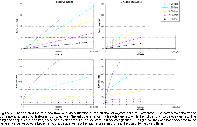
Figure 6 (top left) shows the tree build times for the single node queries with p=128. The times for p=256 are nearly indistinguishable, because the number of nodes in the tree doesn't depend on p (except when a is very small, 1 or 2 in this case). We expect O(ar log r) time, but the data looks very close to linear in r and reasonably close to linear in a. The absolute times are within our 10 second goal up to, e.g., 3 sliders and 200,000 objects, but rise to several times worse for more sliders and objects.

Figure 6 (bottom left) shows the query times for the same parameters. For 1 and 2 attributes, the tree size is limited by p^a rather than the number of objects, so the query time is constant. For 3 attributes, the time grows slowly and is fast enough for interactive feedback with up to a million objects. With 4 attributes the time climbs from tolerable at 50,000 and 100,000 objects to intolerable above 200,000. With higher CPU performance and more memory, we would eventually reach the flatter part of the curve and beat the algorithms that are linear in both a and r. But for now, the TBS algorithm fares better for 4 or more attributes.

In comparing our kd-tree algorithm to TBS, we are comparing the step that causes the bottleneck in each case. For us it is mouse-move, while for TBS it is mouse-down. Since 10x more time is available at mouse-down, kd-trees have to be 10x faster in order to be preferred.

Increasing the histogram width to 256 pixels moved each curve up by a constant amount (not shown). This is due to the large overhead incurred in passing data among Visage, its Java API, and the C code that the kd-trees are implemented in, as well as rendering time in Visage. This overhead is about 20ms per attribute with 128 bucket histograms, and 30ms per attribute with 256 bucket histograms, for both 1 node and 2 node queries. So by the time we have 5 attributes, the goal update time is already used up in overhead before we even look at the data. On top of this constant difference between the 128 bucket and 256 bucket cases, the increase we expect from the complexity formula O(ap^1/(1-a)r^1-1/(1-a)) is not noticeable.

Figure 6 (top right) shows the tree build times for 2 node queries. As expected, they require a constant factor (about 2x) more time than 1 node queries due to the larger memory requirements. The bit vectors add 98 bytes to each tree node, which translates into 6x more memory for 5 attributes. Due to the increased space requirements, we were not able to collect data for the full range of parameter values shown for the 1 node case.

Figure 6 (bottom right) shows the query times for 2 node queries. If we subtract the constant overhead, it appears that there is a constant factor penalty (about 1.7x) over the 1 node case, as expected. This is due to the increased complexity of 64 ORs rather than 1 PLUS. However kd-trees are relatively better here, because the alternative is the Ioannidis approach. kd-trees are surely a win with up to 4 attributes. Even with 5 and 6 attributes they are considerably better than our implementation of the Ioannidis approach.

The complexity analysis and the experiments reported above are for the worst case data distributions. We have anecdotal evidence that the average case is considerably better than this. It suggests that kd-tree algorithms are better than the linear algorithms for a larger number of sliders. We used data from the 1990 Census of Population and Housing for the New England and Mountain states [11]. This data contains 22 attributes about 481K census blocks. We selected the 5 attributes listed in Table 1 for examination in VQE. These were picked because they seemed intuitively interesting and independent of one another.

The resulting kd-tree contained only 161K leaf nodes, a third of the number of objects, because the data is far from uniformly distributed and independent. Many of the histograms had only 1 or 2 bars whose height was noticeably above zero. For instance, a few census blocks had a land area in the hundreds of thousands, while 90% of the areas were less than 100. Thus well over 90% of the distribution was shown in a single histogram bar. Moving the sliders was extremely fast, but also not very interesting. We set the ranges of each slider to minimally enclose the bulk of the distribution, as indicated in Table 1 (middle

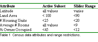
column). We made this a new active subset, now containing 238K objects with interesting distributions across all 5 attributes. The resulting kd-tree has 228K leaf nodes, nearly as many as there are objects.

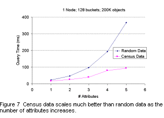
Figure 7 shows the time required to move the latitude slider over 80% of its range, while the other sliders restricted their range as shown in Table 1 (right column). The growth is approximately linear, and much better than that found for independent uniformly distributed data. In fact, the curve for census data is almost indistinguishable from that with random data for 1000 objects. That is, the constant overhead per slider due to message passing and rendering overwhelms any time actually spent in the kd-tree! If this behavior is typical of other real datasets, it makes kd-trees at least competitive with linear approaches for single object queries. It should therefore dominate for multi-object queries.

4. Future Work

4.1. Attributes of Dynamic Aggregates

It is often useful as well to see attributes of dynamic aggregates as their definition changes. For instance we might want to see the average price of houses owned by people in different age brackets, and observe how these averages change as the boundaries between age brackets is varied. If we were interested in the count of houses owned by people in different age brackets this could be done using the kd-tree algorithm. Every time we move the mouse to adjust the boundaries we compute new histograms. In the single object case we can store summary attributes at each tree node in order to compute “histograms” of sums, averages, minimums, and maximums for any attribute. In the multiple object case we can still compute minimums and maximums this way, since including duplicate objects does not change the result. For sums and averages we would use `bit vectors’ where the stochastically encoded value for an object is the attribute value rather than the constant 1 used for counting.

4.2. Efficient Query Previews

For these DQ algorithms to execute within the time limits given in Section 1.1, the data must reside in main memory. In order to explore datasets of terabytes that reside on network servers, subsets must be downloaded to the local machine. Query Previews [12] is an interface similar to DQ histograms to choose range restrictions on a number of attributes that result in a subset of appropriate size. At data warehouse update time an array of dimensionality a is built with an element for every possible combination of attribute values. This is closely related to the Datacube structure used for materializing database queries [13]. Here, the attributes must be quantized to a small number (e.g. Q = 20) levels and then a large array containing counts for all Q^a combinations of attribute values is stored instead of the data. This has the problem of enormous memory for large Q or a, and in some cases, counts for individual bars in the histogram might need to be built from millions of table entries.

Instead we can take advantage of AD-trees [14], a new data structure that allow constant-time counting (independent of number of records) for datasets with nominal values. They have the same functionality as datacubes and Query Previews except that they avoid storing redundant information and use the algebra of contingency tables to save memory. In some cases (e.g. a birth-outcomes data warehouse) they reduced the amount of memory needed to store a 100-dimensional datacube from 10³⁸ down to 10⁶ bytes. Recent work on Lazy AD-Trees [15] preliminarily provides much bigger savings, and may allow constant time querying for up to about 10 attributes each with as many as 30 values. Unfortunately querying involves a subtraction step, so in their present form AD-trees can not be used with bit vectors for multi-object previews.

5. Conclusion

We have presented an overview of precomputed index structures for efficient dynamic query histograms, and described three new theoretical contributions. We verified these ideas experimentally, and compared the performance to previous systems.

First, we showed how to modify existing algorithms to work with multi-object queries. The modification uses an algorithm due to Flajolet and Martin for counting the number of unique values in a database. Exponentially distributed hashed bit vectors are used to approximately represent sets of unique objects.

Second, we presented a theoretical complexity analysis of kd-trees for computing histograms, concluding that the asymptotic behavior is no better than sequential scanning.

Third, we proposed building separate kd-trees for each histogram bucket, and showed that the asymptotic behavior scales better than sequential scanning as the number of objects increases, but worse as the number of attributes increases.

Using single object queries, experiments show that having a kd-tree for each histogram bucket indeed generates histograms much faster than using a single tree. On random data, experiments also verified the relationship between kd-trees and sequential scanning. With a few hundred thousand objects, they are faster than sequential scanning for up to three attributes. The improvement in theoretical complexity will translate into an advantage for more attributes as the computing capacity to explore larger datasets becomes available. There is evidence that kd-trees are faster on real data at least up to 5 attributes.

For multi-object queries, the kd-tree algorithm incurs a constant factor penalty in both space and time to store and process the array of bit vectors, rather than single integers. The overhead of the tree structure itself partially masks this effect. We observed only a 2x slowdown in tree construction and a 1.7x slowdown in histogram calculation. With 5 attributes, the tree took about 6x as much space as in the single object case. These penalties seem quite acceptable.

The subtraction step of the TBS algorithm does not work with the bit-vector representation as used in multi-object queries, and working around this problem probably makes the algorithm slower than direct computation of histograms at mouse-move time.

The pointer chasing approach for multi-object queries produces exact counts rather than estimates, and does not incur the space penalty of bit vectors. Its histogram building time scales linearly in both the number of attributes and the number of composite objects. Based on our previous experience with this approach, we believe the algorithm presented in this paper performs much better for the range of parameters examined here.

Acknowledgments

This work was supported by DARPA contract DAA-

1593K0005. We greatly appreciate Stephan Kerpedjiev’s helpful comments on an earlier draft. Christos Faloutsos led us to the literature on approximate counting algorithms.

References

[1] M. Derthick, J. A. Kolojejchick, and S. Roth, “An Interactive Visual Query Environment for Exploring Data,” presented at Proceedings of the ACM Symposium on User Interface Software and Technology (UIST), Banff, Canada, 1997, p. 189-198.

[2] S. F. Roth, M. C. Chuah, S. Kerpedjiev, J. A. Kolojejchick, and P. Lucas, “Towards an Information Visualization Workspace: Combining Multiple Means of Expression,” Human-Computer Interaction Journal, vol. 12, pp. 131-185, 1997.

[3] C. Ahlberg, C. Williamson, and B. Shneiderman, “Dynamic Queries for Information Exploration: An Implementation and Evaluation,” presented at Human Factors in Computing Systems (CHI), Monterey, CA, 1992, p. 619-626.

[4] E. Tanin, R. Beigel, and B. Shneiderman, “Design and Evaluation of Incremental Data Structures and Algorithms for Dynamic Query Interfaces,” presented at Proceedings of the IEEE Information Visualization Conference (InfoVis), Phoenix, AZ, 1997, p. 81-86.

[5] J. L. Bentley, “Multidimensional binary search trees in database applications,” IEEE Transactions on Software Engineering, vol. 4, pp. 333-340, 1979.

[6] D. T. Lee and C. K. Wong, “Quintary Trees: A File Structure for Multidimensional Database Systems,” ACM Transactions on Database Systems, vol. 5, pp. 339-353, 1980.

[7] V. Jain and B. Shneiderman, “Data Structures for Dynamic Queries: An Analytical and Experimental Evaluation,” University of Maryland, College Park, MD, Technical Report CAR-TR-685, September 1993.

[8] R. Beigel and E. Tanin, “The Geometry of Browsing,” presented at Latin American theoretical informatics (LATIN), 1998, p. 331-340.

[9] Y. Ioannidis, “Dynamic information visualization,” SIGMOD record, vol. 25, pp. 16-20, 1996.

[10] P. Flajolet and G. N. Martin, “Probabilistic Counting,” presented at Foundations of Computer Science, 1983, p. 76-82.

[11] United States Bureau of the Census, “Census of population and housing,” , 1990.

[12] K. Doan, C. Plaisant, and B. Shneiderman, “Query Previews in Networked Information Systems,” presented at Research and technology advances in digital libraries, Washington; DC, 1996, p. 120-129.

[13] V. Harinarayan, A. Rajaraman, and J. D. Ullman, “Implementing Data Cubes Efficiently,” presented at Proceedings of the Symposium on Principles of Database Systems (PODS), 1996, p. 205-216.

[14] A. W. Moore and M. S. Lee, “Cached Sufficient Statistics for Efficient Machine Learning with Large Datasets,” Journal of Artificial Intelligence Research, vol. 8, 1998.

[15] P. Komarek and A. W. Moore, “Lazily Cached Sufficient Statistics: New data structures and theory,” In preparation, 1999.